Currents:

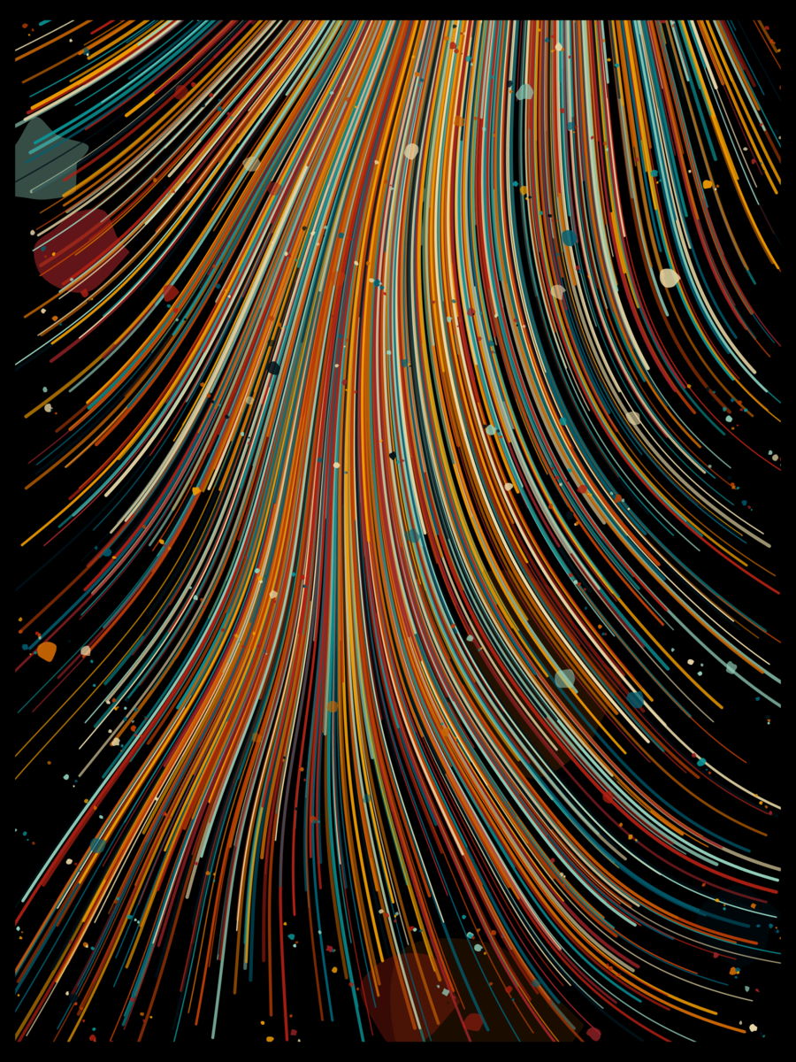
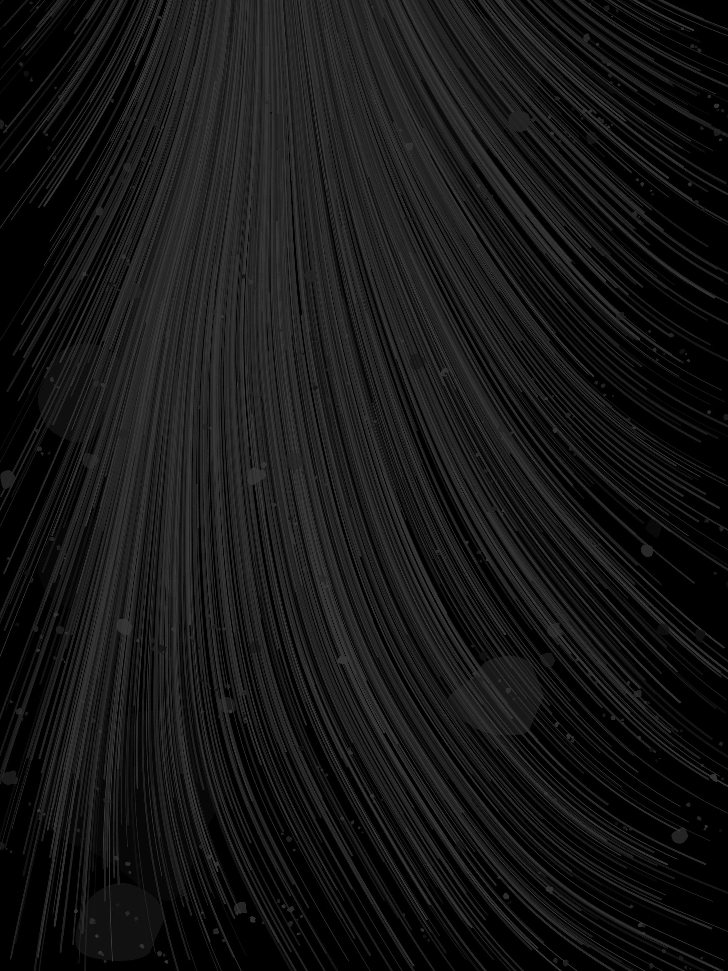
Currents are a long form generative art collection written in p5.js that employs flow fields and Fibonacci stepping for detailed, aesthetic visuals of fluid dynamics.

Currents arose out of a desire to visually express the propagation of Constructs across social and historical substrates.

The ability for ideas to flow freely within our society, in my mind, emulates the movement of water closely, hence the subject matter and title of the work.

Currents are composed of 10 primary attributes: Background, Palette, Turbulence, Stroke Density, Stroke Thickness, Stroke Length, Stroke Variance, Drip Density, Drip Size, and Chopped.

The algorithm begins by creating the canvas and selecting a palette and the Turbulence level of the piece.

Currents are 2520x3360 (3:4 Aspect Ratio) and utilize 4 different Turbulence values (Flowless, Rough, Standard, and Smooth).

The selected Turbulence level determines the directionality, velocity, and force which the underlying flow field assumes.

After this is done, the remainder of the metadata is generated to guide the algorithm as it paints the canvas.

The metadata is selected based on a custom normal random weighted distribution algorithm written expressly for use in my work.

All probabilities, for every attribute, in the work, are Fibonacci values. This technique is utilized to produce natural, aesthetic attribute proportionality across the entire work and not simply within individual pieces.

The generated metadata is then put through an exception filter that defines combinations that should never appear in tandem to produce a more curated aesthetic based on my own personal preferences from prior outputs while developing the algorithm.

I generated approximately 150,000 images over a span of about a month and a half during the development of this work.

The conflicting attributes, should a conflict arise, are re rolled if necessary.

The background is the first thing painted on the canvas.

The background is a hex value correlated with the value of the Background trait unless the background trait was rolled as “Palette”. If the Background trait is rolled as “Palette”, the algorithm selects, at random, a color from the selected palette, however, because this color must be opaque, a modification is made to the selected color itself (without modifying the instance of the color that exists within the palette) to ensure it’s opacity is maxed, as other colors selected from the palette may have their opacity modified when picked to increase depth in the work.

Next the algorithm runs another exception filter on the Stroke Density, Stroke Thickness, Stroke Length, and Stroke Variance attributes to determine whether or not a conflict exists between any of these attributes based on the curation of prior generations. Should this check fail, the conflicting attributes are re rolled until no conflict exists.

There are no exception filters on Drip Density, Drip Size, or the Chopped attribute values.

Once the metadata is complete, the primary draw method begins.

The draw function of Currents is comprised of 10 loops that draw elements on the canvas according to their size.

We begin this function by defining an array that is going to store all of the coordinates for our "drips”, the circular shapes haphazardly painted on the canvas to provide texture and variation to the resulting piece.

We define this array to utilize the circumference and coordinates of the circle, to do basic collision detection to ensure we do not allow drip intersections that might be aesthetically unsavory.

We start with the largest circular drips drawn on the canvas. These drips are drawn at random locations on the canvas with no respect to the flow field. They are the only drips in the algorithm that do not respect the flow field and the reason for doing this is to increase variation and inject a bit of controlled chaos. The frequency of these drips is dictated by a combination of the Drip Density attribute divided by the product of two constant Fibonacci values.

The size of these drips is also Fibonacci stepped. The size is determined by the same two Fibonacci values used to determine the frequency multiplied by the Drip Size selected when the metadata of the piece was generated.

Once these values are set, the coordinates of the new drip are compared against existing drips within the array set up at the beginning of the function to determine if any color overlap occurs. Should overlap occur, the color selected is re rolled until no conflicting overlap exists.

Finally, the opacity for this degree of drip is set to a more translucent value than any subsequent drips drawn on the canvas. The opacity value is selected at random from within a predefined range.

Finally, we begin to draw the actual drip.

First, to increase variation in the drips, we generate a number that will determine the number of sides the circular object will contain. This value is selected at random from within a pre defined range.

Once this value is set we create vertices guided by the number of sides / edges we previously set to draw each side of the drip individually. Finally, we close the shape and fill it with the color we determined within the primary draw function.

As previously mentioned, we let this loop run until our increment exceeds the value we set via by dividing the Drip Density by the product of the two static Fibonacci values that control this portion of the primary draw function.

Once our large drips have been painted on the Canvas, we begin drawing our largest lines.

Our largest lines follow a similar overall pattern to how the drips are painted, however, with their own unique constraints and implementation details. Once again, we create random x, y coordinates, ensuring we are not using a color that would be invisible due to being the same as the background, and guide the loop by using Fibonacci to step the values that control how many times the loop drawing these lines will run, and also the individual length and thickness multipliers that will be applied to the lines drawn within this specific loop of the draw function. Similarly to the drips, we define an opacity range and apply it to the color we’ve picked from the palette. One of the primary differences between this and the prior loop is that the shapes drawn by this loop get drawn with directionality and force applied via the underlying flow field we set up at the beginning of the algorithm.

It is important to note that when creating pieces like this, controlling the flow field is extremely important.

Too much noise, too much variability, too much directionality, too high or low of a resolution for the grid, can all have disastrous results for the piece.

Inside of our draw function, a different function where the line drawing logic exists will be called, we select a starting point for the line based on the x, and y coordinates we generated in the main draw function and the field resolution we initially set for the flow field as a constant at the top of the algorithm. We then multiply our Line Variance attribute (which contains an array of different Fibonacci values depending on the value this trait is set to) by our Line Thickness to determine the stroke the individual instance of the line will have. Once this is complete, we begin drawing the line by observing its length and moving across the flow field using our x and y coordinates as an index to track the underlying grid. One of the last things we due in this step is modify the result of the product of Line Variance and Line Thickness by using a Perlin Noise function to constrain the adjustment stepping as we traverse the flow field.

We stop drawing the line when the Line Length for this particular line is reached.

These two processes described for drawing both the lines and the drips occur 8 more times in much the same way, with different Fibonacci values governing the individual runs. Progressively, smaller and smaller lines and drips are drawn as we move through the main draw function.

The lines and drips are drawn in different orders to simulate depth and increase variation.

The only notable change that occurs towards the end of the algorithm is a spatter algorithm is used to guide the last 4 drip loops that occur. This portion of the algorithm, once again, uses fibonacci values to determine how close certain drips are to one another on the canvas and groups them along the flow field to emulate how spatter patterns work in nature.

Finally, once the main draw loop completes, a frame is drawn on top of the canvas.

The frame color is dependent on the Background trait selected.

White backgrounds inherit white frames.

Black backgrounds inherit black frames.

Palette and Cream backgrounds inherit the darkest color of the palette that is selected by converting the entire palette from hex values to HSL values and calculating the luminance of each individual color within the palette.

And without droning on for too long, that is essentially how I wrote Currents. I had a lot of fun writing this algorithm. It took roughly 250-300 hours of actual coding and the process spanned roughly a month and half. This is excluding curation of the resulting pieces to ensure only the highest quality outputs for collectors of the work. In total, I’d estimate this algorithm took me somewhere in the ball park of 450-500 hours including curation. That all equates to an average time spent of 10-12 hours per day for roughly 45 days straight. The final code is roughly 1,000 lines after optimization and I can proudly state it is the best work I’ve ever produced.

They launch March 1st for .5 SOL (roughly 52 USD at the time of this writing) on Truffle.

Alongside this blog post, you will find samples of the work.

Thank you for your time.